Notebooks

Evaluating Clustering Performance

NOTE: Most of this notebook's content is adapted—often copied!—from scikit-learn's excellent documentation on clustering. This is a compilation of definitions and code-snippets that I found useful while working on a project, along with some of my own thoughts.

Evaluation of quality of clusters is often done in two ways:

• comparing how well the predicted clusters compare with the ground truth and
• checking if the generated clusters are consistent.

The second approach is the only option if no ground truths are available.

There are several coefficients that quantify the quality of clustering. Some that do not need a ground truth are Silhouette coefficient, Calinski–Harabasz index, and Davies–Bouldin index. Others such as homogeneity Score, completeness score, and V Measure need a ground truth.

Silhouette coefficient

For a single sample it is

$$ s = \frac{b - a}{\max(a, b)}. $$

• $a$: mean distance between a sample all other points in the same cluster
• $b$: mean distance between a sample all other points in the next nearest cluster.

$s$ takes values in $[-1,1]$ with

• $-1$ meaning incorrect clustering,
• 0 meaning overlapping clusters, and
• 1 meaning highly-dense, well-separated clusters.

So, a higher silhouette score means better defined clusters.

Important: Scikit returns the mean of all Silhouette coefficients of the samples.

Scikit mentions a drawback:

The Silhouette Coefficient is generally higher for convex clusters than other concepts of clusters, such as density based clusters like those obtained through DBSCAN.

Calinski Harabasz Index

Calinski–Harabasz index (CHI) is the ratio of the sum of between-clusters dispersion for all clusters and sum of inter-cluster dispersion for all clusters. Better-defined clusters have higher CHI value.

Davies-Bouldin Index

Surprisingly, DB values closer to zero indicate a better partition, unlike Calinski-Harabasz index and Silhouette coefficient.

For CHI and DBI formulas, check the referenced scikit doc page.

Homogeneity Score

Homogeneity score ($h$) is defined as $$ \begin{align*} &h = 1 - \frac{H(C|K)}{H(C)}\;\text{where}\\ &H(C) = - \sum_{c=1}^{|C|} \frac{n_c}{n} \cdot \log\left(\frac{n_c}{n}\right)\\ &H(C|K) = - \sum_{c=1}^{|C|} \sum_{k=1}^{|K|} \frac{n_{c,k}}{n}\cdot \log\left(\frac{n_{c,k}}{n_k}\right) \end{align*} $$

• $n$: total number of samples.
• $n_c$, $n_k$: number of samples in class $c$ and cluster $k$, respectively.
• $n_{c,k}$: number of samples from class $c$ assigned to cluster $k$.

Higher $h$ means better clusters. $h$ takes values in $[0,1]$.

Completeness Score

• All members of a class belongs to the same cluster.
  • $c = 1 - \frac{H(K|C)}{H(K)}$
  • $c \in[0,1]$. higher is better.

V-Measure

• The harmonic mean of the homogeneity score and completeness scores: $v = 2 \cdot \frac{h \cdot c}{h + c}$.
• It's implemented in scikit as $v = \frac{(1 + \beta) \times \text{homogeneity} \times \text{completeness}}{(\beta \times \text{homogeneity} + \text{completeness})}$

from sklearn import metrics
labels_true = [0, 0, 0, 1, 1, 1]
labels_pred = [0, 0, 1, 1, 2, 2]

print(metrics.homogeneity_score(labels_true, labels_pred))
print(metrics.completeness_score(labels_true, labels_pred))
print(metrics.v_measure_score(labels_true, labels_pred, beta=0.6))

0.6666666666666669
0.420619835714305
0.5467344787062375

Mutual-information-based similarity score

Let's say, we have 2 sets of labels, $U$ and $V$, for $N$ objects. If $P(i)=|U_i|/N$ and $P'(j)=|V_i|/N$ are the probabilities that a randomly-picked object from $U$ ($V$) falls into class $U_i$ ($V_j$), then the entropies and the mutual information between $U$ and $V$ are computed as $$ \begin{aligned} H(U) &= - \sum_{i=1}^{|U|}P(i)\log(P(i))\\ H(V) &= - \sum_{j=1}^{|V|}P'(j)\log(P'(j))\\ \text{MI}(U, V) &= \sum_{i=1}^{|U|}\sum_{j=1}^{|V|}P(i, j)\log\left(\frac{P(i,j)}{P(i)P'(j)}\right)\\ &= \sum_{i=1}^{|U|} \sum_{j=1}^{|V|} \frac{|U_i \cap V_j|}{N}\log\left(\frac{N|U_i \cap V_j|}{|U_i||V_j|}\right)\\ \text{NMI}(U, V) &= \frac{\text{MI}(U, V)}{\text{mean}(H(U), H(V))}\\ \text{AMI} &= \frac{\text{MI} - E[\text{MI}]}{\text{mean}(H(U), H(V)) - E[\text{MI}]} \end{aligned} $$

• AMI is adjusted against chance. NMI and MI are not.
• AMI
  • $<0$: bad (i.e. independent labeling)
  • $=0$ (random labeling)
  • $\simeq 1$ (agreement between the ground truth and predicted labels)

References:

• C. D. Manning, P. Raghavan, H. Schütze. Introduction to Information Retrieval; Cambridge University Press: New York, 2008. pp. 356–359 (Good discussion.)

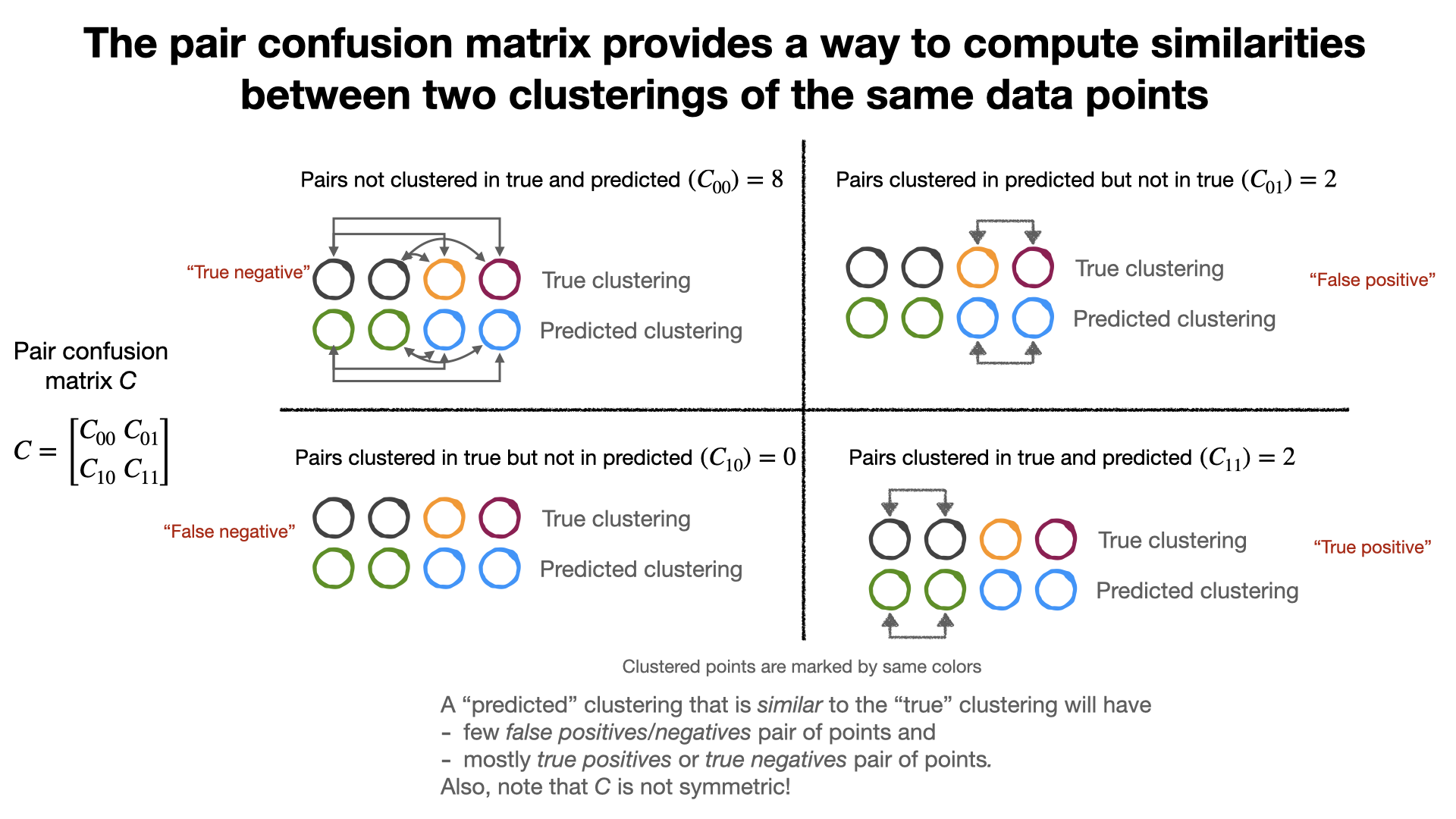
Pair confusion matrix

Two clusters can be compared using the pair-confusion Matrix.

from sklearn.metrics.cluster import pair_confusion_matrix
from sklearn import metrics
import numpy as np
C = pair_confusion_matrix([0, 0, 1, 1], [0, 0, 1, 2])
print(C)
TN = C[0, 0]
FP = C[0, 1]
FN = C[1, 0]
TP = C[1, 1]

[[8 0]
 [2 2]]

Fowlkes–Mallows Index

Building on the pair-confusion matrix, FMI, a measure for cluster similarity, is computed using the elements of $C$ as $$FMI = \frac{TP}{\sqrt{(TP + FP) (TP + FN)}}.$$

FMI is useful because it gives a number—and not a matrix like the pair confusion matrix—for quickly comparing two clusterings.

FMI = TP / np.sqrt((TP + FP) * (TP + FN))
print(FMI)
# You Can also Compute FMI Using Scikit-learn. The Results Match, of Course.
print(metrics.fowlkes_mallows_score([0, 0, 1, 1], [0, 0, 1, 2]))

# Also Two Same Partitions Will Have no Off-diagonal Elements in the Pair Confusion Matrix and a FMI Score of 1.

C = pair_confusion_matrix([0, 0, 1, 1], [0, 0, 1, 1])
print(C)
TN = C[0, 0]
FP = C[0, 1]
FN = C[1, 0]
TP = C[1, 1]

FMI = TP / np.sqrt((TP + FP) * (TP + FN))
print(FMI)

print(metrics.fowlkes_mallows_score([0, 0, 1, 1], [0, 0, 1, 1]))

0.7071067811865475
0.7071067811865476
[[8 0]
 [0 4]]
1.0
1.0

Element-centric similarity and issues with FMI and NMI

Gates et al. raise objections against using Fowlkes–Mallows Index and NMI, specifically NMI; they proposed a new one.

References:

• A. J. Gates et al. Element-Centric Clustering Comparison Unifies Overlaps and Hierarchy. Sci Rep 2019, 9 (1), 8574. DOI.
• A. J. Gates, Y.-Y. Ahn. CluSim: A Python Package for Calculating Clustering Similarity. Journal of Open Source Software 2019, 4 (35), 1264. DOI.
• https://github.com/Hoosier-Clusters/clusim of Gates et al. with their package

from clusim.clustering import Clustering
import clusim.sim as sim

true_labels = [1, 1, 1, 2, 2, 2, 3, 3, 3]
predicted_labels = [1, 2, 2, 3, 3, 1, 1, 1, 1]
single_cluster_labels = [1, 1, 1, 1, 1, 1, 1, 1, 1]
completely_fragmented_labels = [1, 2, 3, 4, 5, 6, 7, 8, 9]

# Their Data is Differently Formatted.
true_clustering = Clustering().from_membership_list(true_labels)
predicted_clustering = Clustering().from_membership_list(predicted_labels)
predicted_single_cluster = Clustering().from_membership_list(single_cluster_labels)
predicted_completely_fragmented = Clustering().from_membership_list(
    completely_fragmented_labels
)

for _ in [
    predicted_clustering,
    predicted_single_cluster,
    predicted_completely_fragmented,
]:
    print(
 f"FMI = {sim.fowlkes_mallows_index(true_clustering,_)}, NMI = {sim.nmi(true_clustering,_)}, elem-cent = {sim.element_sim(true_clustering,_)}"
    )
# The Package Can Compute Many Scores such As... (code from Their Documentation https://hoosier-clusters.github.io/clusim/html/clusim.html)

row_format2 = "{:>25}" * (2)
for simfunc in sim.available_similarity_measures:
    print(
 row_format2.format(
     simfunc, eval("sim." + simfunc +
"(true_clustering, predicted_clustering)")
 )
    )

FMI = 0.4811252243246881, NMI = 0.5451600159416435, elem-cent = 0.5407407407407406
FMI = 0.5, NMI = 0.0, elem-cent = 0.33333333333333326
FMI = 0.0, NMI = 0.6666666666666665, elem-cent = 0.33333333333333326
            jaccard_index                   0.3125
               rand_index       0.6944444444444444
            adjrand_index      0.26666666666666655
    fowlkes_mallows_index       0.4811252243246881
                 fmeasure      0.47619047619047616
             purity_index       0.7777777777777777
     classification_error      0.22222222222222232
        czekanowski_index      0.47619047619047616
               dice_index      0.47619047619047616
           sorensen_index      0.47619047619047616
    rogers_tanimoto_index       0.5319148936170213
          southwood_index      0.45454545454545453
      pearson_correlation      0.00102880658436214
         corrected_chance      0.16994265720286564
      sample_expected_sim      0.10526315789473684
                      nmi       0.5451600159416435
                       mi       0.8233232815796736
                   adj_mi       0.3410389011275906
                      rmi       0.1464053299155769
                       vi       1.3738364418444755
       geometric_accuracy       0.7777777777777778
          overlap_quality                     -0.0
                     onmi       0.6303315236619905
              omega_index      0.26666666666666655